Demand Forecasting (part 1)

Introduction

This blog series are about demand forecasting in D365FO. I will explain different parameters and forecasting methodologies and explain how to use Azure Machine Learning to forecast demand in F&O.

When I talk about demand forecasting, I am referring to the process of anticipating future requirements (demand) for products using different methodologies. Demand is any request to deliver goods, either to end customer or for consumption in production.

Demand forecasting is used to predict future demand that can either be independent, such as demand from sales orders (thus demand for finished goods), or dependent, such as demand that is created as demand for production components. Dependent demand can usually be derived from bills of materials.

Demand forecasting is, though always containing a level of uncertainty, a very important source of information used in business decisions. Demand forecasting helps:

• Reduce buffer stock: with more accurate demand forecast, companies can reduce buffer stock, thus reducing the amount of cash tied up in that stock.
• Eliminate or mitigate risks related to purchasing and lead times: demand for items with long lead time can be forecasted and those can be procured or produced in time to supply real demand when it occurs. Demand forecasting allows you to gain early insight into the demand for products. This allows you to purchase on time and prevents your supplier from being sold out.
• Increase revenue: anticipating demand can impact purchasing strategies and therefore can lead to more favourable contracts with vendors. On the sales side, especially in retail, customers need to have goods available to them when they need them, otherwise company loses sales
• Anticipate capacity demand: when demand is forecasted, production resources can be planned and scheduled to meet increased demand. This can have significant demand on business decisions
• Provide insight in budget and future cash flow: demand can indicate when increased cash demand will be created and drive business decisions around budgeting and cash flow

And more…

Methodologies

There are many methodologies to predict future demand, but in general, they are split in three major principles:

• Time series: forecast is based on historical data. This methodology is mostly used when there is enough historical data, usually in well established businesses.
• Qualitative analysis: this method relies on expert opinions, market research et., and it is used when there is scarce historical data available. It is usual in new businesses or when new product is introduced in the market.
• Causal models: this method is most complex but also most sophisticated and relies specific information about relationships between variables affecting demand in the market, such as competitors, economic forces, and other socioeconomic factors. As with time series analyses, historical data is key to creating a causal model forecast.

Some math (just a little bit of)

As said, forecast is never 100% accurate. However, we need to know how good the forecast is. As with anything else, some math jumps in to help us out. Accuracy of demand forecast is measured by MAPE. This stands for Mean Absolute Percent Error and behind this complex name simply hides an average percentage of error we made for every forecasted value. The formula to calculate MAPE is:

where _At is the actual value and _Ft the forecast value. Their difference is divided by the actual value A_t. The absolute value in this ratio is summed for every forecasted point in time and divided by the number of fitted points n. Let’s look at example below and explain what MAPE means:

Here, red arrows represent deviation of forecast from actual values. Based on the data MAPE is 1,31%. This means our forecast is, on average, off by 1,31% (pretty good, right?).

How does forecasting process work in D365 F&O?

D65FO uses Time series methodology to forecast demand. This means it relies on historical data to forecast future demand. For forecasting purpose, we assume that time series data is time dependent and that it demonstrates certain patterns or characteristics.

Time series forecasting relies on historical data as source used to produce forecast of demand. Time series are made up of four following components or variables:

• Trend. The increasing or decreasing behaviour of the series over time, often linear. Think about increasing demand for electric cars.
• Seasonality: Repeating patterns or cycles of behaviour over time. Think of increased demand for sunscreens during summer.
• Cyclic behaviour: this sort of behaviour occurs when data exhibits rise or fall that do not have fixed frequency. This is different from seasonality because seasonal patterns do have regular frequency.
• Error: this is variability series that cannot be explained by the model. Think of huge once-in-a-lifetime order for bike tires by the customer.

Later will we see which parameter determines how these characteristics are accounted for.

Forecast generation strategies

There are three forecast generation strategies available to forecast future demand in D365FO:

• Copy over historical demand
• Azure Machine Learning Service
• Azure Machine Learning

However, the reason for having three is because the last option, Azure Machine Learning is a forecast model that uses Azure Machine Learning Studio (classic). However, Azure Machine Learning Studio (classic) has been deprecated and will soon be removed from Azure, so Microsoft recommends selecting Azure Machine Learning Service if you’re setting up demand forecasting for the first time or plan to switch to it if you are already using Azure Machine Learning for forecasting.

Do note that you must enable Azure Machine Learning Service for demand forecasting feature in Feature management to see the second option.

In our blog we will explain how to use all of those, but let’s first explain some parameters.

Demand forecasting parameters

Each of the forecast generation strategies relies on its own set of parameters that I will describe in later chapter, but I will begin with some prerequisites that are required by all of them.

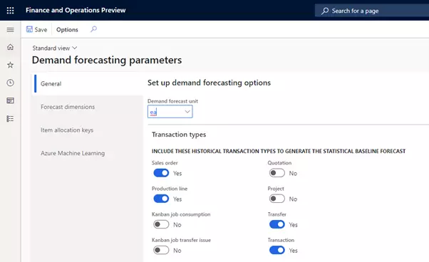
• Demand forecast unit: You can find this in demand forecasting parameters. This is the default unit for forecasting. Having one default forecast unit implies that there needs to be unit conversion to this unit for every item that will be forecasted
• Transaction types: these determine which historical transactions will be considered for generating forecast

Users can choose between Sales orders, Production orders, Kanban jobs (production and transfer), Quotations, regular transfer orders and (other) outbound inventory transactions.

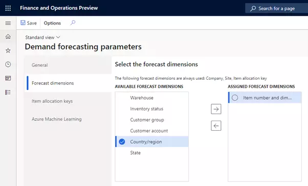
• Forecasting dimensions: you can select dimensions to determine hoe granular your forecast will be. Mind you, that default dimensions that are always used are Company, Site, and Item allocation key. Additional dimensions can be added. Note that item ID is not mandatory. This means forecast can (for example) be done for a group of items, based on Item allocation key.

Tip: start forecasting with fewer dimensions. When demand is forecasted, not only do more dimensions have performance impact, but when historical data is dispersed, this will likely generate more inaccurate forecast.

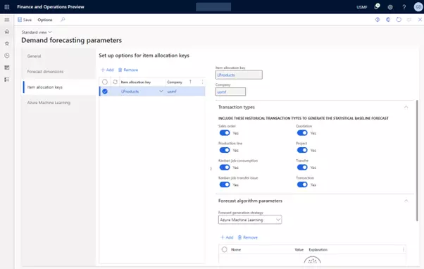
• Item allocation keys: As noted above, item allocation key is mandatory dimension. This implies that you need to assign items to at least one Item allocation key to generate forecast for it.
  – Setup options for item allocation keys: It is possible to set up Item allocation keys to use different transaction types as source but also to use different algorithms:

Granularity attribute

Granularity attribute is a combination of forecast dimensions against which the forecast is done. You can define forecast dimensions on the Demand forecasting parameters page. When forecast is generated, every row of the forecasted data will contain unique combination of the forecast dimension values that are enabled. You can see granularity attribute in Adjusted demand forecast page:

Forecast algorithm parameters

Forecast algorithms in Microsoft Dynamics 365 for Finance and Operations use several parameters. I will explain shortly what each of these means. It is important to understand what behaviour is controlled by these and in which way you can adjust them to generate forecast that is most accurate, or, more correct – less inaccurate.

Forecast generation strategy

We have already explained it above, but it is part of Forecast algorithm parameters

Forecasting model

Forecasting model specifies which forecasting model to use. In D365FO the following models are available. I am providing Wiki links for more details about each because explaining them would require a separate blog for each:

• ARIMA – AutoRegressive Integrated Moving Average (https://en.wikipedia.org/wiki/Autoregressive_integrated_moving_average)
• ETS – Error, Trend, Seasonal (https://en.wikipedia.org/wiki/Exponential_smoothing)
• STL – Seasonal and Trend decomposition using Loess (https://en.wikipedia.org/wiki/Seasonal_adjustment)

The following options instruct the algorithm to use combinations:

• ETS+ARIMA
• ETS+STL
• ALL.

Do note that there is another parameter called Forecast model, and it is not to be confused with Forecasting model. Forecast models will be explained later.

Test set size percentage

Whenever forecast is calculated, system will use part of data set to calculate the forecast, while part of data will be used to test the accuracy of the calculation. For example, setting this parameter to 25% means that 75% of data will be used to calculate forecast, while 25% will be used as a test set for forecast accuracy calculation (MAPE). Overall, around 20% is the good value to start with. Larger values can also have performance impacts.

Confidence level percentage

A confidence interval indicates what is the confidence interval. The confidence interval represents a range of values that we think our demand might fall in. These values act as good estimates for the demand forecast. For example, a 95% confidence level percentage indicates there is a 5% risk that the future demand falls outside the confidence interval range. The greater the value of confidence level percentage, the greater the area that we assume demand will fall in. The parameter ranges from 1 to 99. This value impacts how we view the forecast, but not the actual forecast values themselves. The results can be seen in Adjusted demand forecast page:

Minimum (and maximum) forecasted value

This number indicates what the system should use as minimum of maximum forecasted value. For example, let’s assume the system does not foresee any demand for selected item and period. In this case, forecast would normally return 0. However, if we set minimum value to 1, this will then be returned as forecasted value. Similar applies to maximum value: imagine the system forecasts demand for 156 pieces of specific item in a specific period, but we set maximum value to 150. In this case, forecasted value will be topped at 150.

Missing value substitution

This parameter specifies what should happen if there are gaps in historical data. It indicates how these gaps are to be filled. The following options can be selected: (numeric value),

• MEAN – average value for previous and following data points would be inserted as substituted value
• PREVIOUS – previous value will be inserted as substituted value
• INTERPOLATE LINEAR – interpolated value will be calculated using linear interpolation and inserted as substituted value.
• INTERPOLATE POLYNOMIAL – interpolated value will be calculated using polynomial interpolation and inserted as substituted value.

Missing value substitution needs to be carefully considered. It can happen that the value is missing because there actually was no demand – so you would not want to just insert some value as substitute; instead, in this case – it would be zero.

Missing value substitution scope

Paired with missing value substitution is the parameter that determines the scope of the missing value substitution. This parameter decides whether the value substitution applies only to the date range of each individual granularity attribute, or to the entire dataset. The following options are available for establishing the date range that the system uses when filling in gaps in historical data:

• • GLOBAL – The missing values will be replaced using the missing value substitution method in the whole historical data range used for calculating forecast.
  • HISTORY_DATE_RANGE – The system will substitute data within a specific date range that we set when we run Generate statistical baseline forecast. This range is defined by the From date and To date fields In the Historical horizon section.
  • GRANULARITY_ATTRIBUTE – The system will substitute data within the currently processed granularity attribute.

In most of the cases, setting this parameter to GLOBAL is the best option.

Force seasonality

This parameter applies to ARIMA and ETS forecast models only. It specifies what the relationship between trend and seasonality is. Setting this parameter tells the system whether to force the model to use a specific type of seasonality.

The following options are available:

• AUTO (default option)
• NONE – no seasonality pattern will be forced.
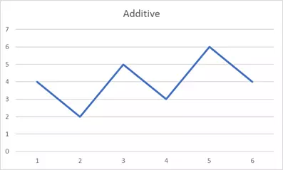
• ADDITIVE – seasonality impact is independent of trend. This indicates that seasonal pattern remains the same and the trend remains the same, independent of each other. For example, there is always increase in demand for sunscreens in the summer months, while the overall trend is growing over the time. While year after year demand is increasing, we will still see peaks in demand during summer, just like in the graph below.

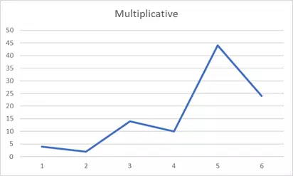
• MULTIPLICATIVE – the seasonality magnitude depends on the trend. This indicates that if there is a growing trend, then seasonal increases or decreases in demand will be multiplied with this growing trend. Example in the graph below

Seasonality hint

As mentioned before, seasonality is one of the characteristics of time series. For seasonal data, we should provide a hint to the forecasting model to improve forecast accuracy. This is done via Seasonality hint parameter which is an integer number that represents the number of buckets that a demand pattern repeats itself for. For example, if there is a repeating pattern every 6 months, and we are forecasting in monthly buckets, then we should enter 6.

Item allocation keys

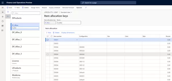
For every item that demand needs to be forecasted, the item needs to be assigned to at least one item allocation key. Items will be assigned to Item allocation keys with product dimensions.

The percentage defined here represents percentage of the total aggregate forecast quantity that you want to allocate to the item. Total percentages can be higher or lower than 100%. Note that during demand forecasting, the item allocation percentages that assign a part of an aggregate forecast to individual items are not used. Item allocation percentages do not affect the demand forecast quantities.

This percentage can be seen only in Net Requirement screen of any of these percentage items in the Item allocation key, you will see these lower-level forecast show up as “demand forecast”.

Forecast model and forecast plan

A forecast model names and identifies a specific forecast. You must create a forecast model before you can create the actual forecast lines. More about forecast model in the following parts of our blog.

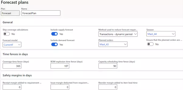
Forecast plan is needed in order to link the master plan with options for forecasting. Most important parameters in forecast plan are time fences and safety margins as well as forecast reduction keys.

We will explain them later when we demonstrate demand forecasting

Outliner removal

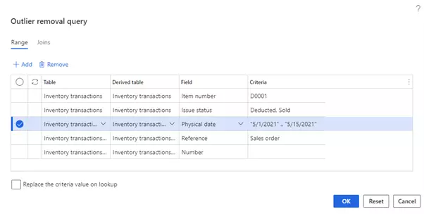
Sometimes there are peaks in historical demand that originate from “once in a lifetime” actions: think about special sales promotions or huge customer orders. These transactions can introduce more inaccuracy in demand forecast. In order to remove such transactions from being considered in forecast calculation D365FO offers Outliner removal functionality. This functionality allows users to build queries that will select transactions to be removed from forecast calculation. For example, If I wish to remove sales during two weeks of May 2021 (when we had a huge promotional campaign), I will create a query indicating sales during that time should be removed:

To review transactions that will be removed from calculation, we can use Display transaction option. This way we can confirm that query returns correct results.

Master plans

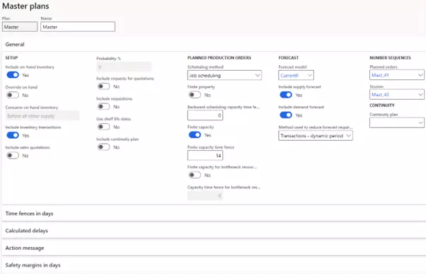
Finally, in order to include forecasted demand as requirement in planning orders generation process, master plans need to be created, and forecast plan needs to be assigned to master plans. Master planning is a separate big topic so we will only mention it here.

End note

This is the first part of our blog. In the second part of our blog, we will cover the topic of Using Azure Machine Learning to forecast demand and in the last one we will demo demand forecasting in Microsoft Dynamics 365 for Finance and Operations.